
Plotting Astropy objects in Matplotlib#
Plotting quantities#
Quantity objects can be conveniently plotted using matplotlib. This
feature needs to be explicitly turned on:
>>> from astropy.visualization import quantity_support
>>> quantity_support()
<astropy.visualization.units.MplQuantityConverter ...>
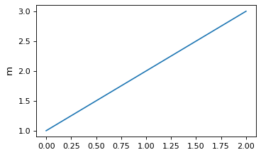
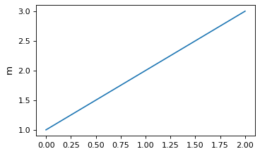
Then Quantity objects can be passed to matplotlib plotting
functions. The axis labels are automatically labeled with the unit of
the quantity:
from astropy import units as u
from astropy.visualization import quantity_support
quantity_support()
from matplotlib import pyplot as plt
plt.figure(figsize=(5,3))
plt.plot([1, 2, 3] * u.m)
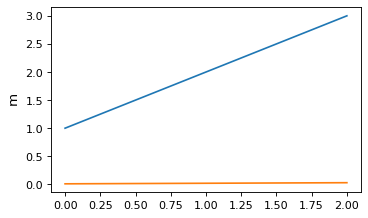
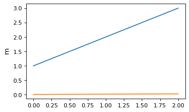
Quantities are automatically converted to the first unit set on a
particular axis, so in the following, the y-axis remains in m even
though the second line is given in cm:
plt.plot([1, 2, 3] * u.cm)
Plotting a quantity with an incompatible unit will raise an exception.
For example, calling plt.plot([1, 2, 3] * u.kg) (mass unit) to overplot
on the plot above that is displaying length units.
To make sure unit support is turned off afterward, you can use
quantity_support with a with statement:
with quantity_support():
    plt.plot([1, 2, 3] * u.m)
Plotting times#
Matplotlib natively provides a mechanism for plotting dates and times on one
or both of the axes, as described in
Date tick labels.
To make use of this, you can use the plot_date attribute of Time to get
values in the time system used by Matplotlib.
However, in many cases, you will probably want to have more control over the
precise scale and format to use for the tick labels, in which case you can make
use of the time_support function. This feature needs to
be explicitly turned on:
>>> from astropy.visualization import time_support
>>> time_support()
<astropy.visualization.units.MplTimeConverter ...>
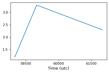
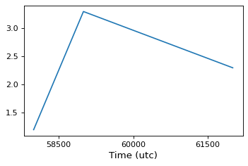
Once this is enabled, Time objects can be passed to matplotlib plotting
functions. The axis labels are then automatically labeled with times formatted
using the Time class:
from matplotlib import pyplot as plt
from astropy.time import Time
from astropy.visualization import time_support

time_support()

plt.figure(figsize=(5,3))
plt.plot(Time([58000, 59000, 62000], format='mjd'), [1.2, 3.3, 2.3])
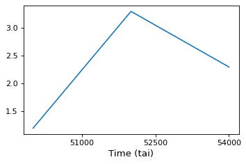
By default, the format and scale used for the plots is taken from the first time
that Matplotlib encounters for a particular Axes instance. The format and scale
can also be explicitly controlled by passing arguments to time_support:
time_support(format='mjd', scale='tai')
plt.figure(figsize=(5,3))
plt.plot(Time([50000, 52000, 54000], format='mjd'), [1.2, 3.3, 2.3])

To make sure support for plotting times is turned off afterward, you can use
time_support as a context manager:
with time_support(format='mjd', scale='tai'):
    plt.figure(figsize=(5,3))
    plt.plot(Time([50000, 52000, 54000], format='mjd'))